Simple Trunks
Examples of MBTA Bus Routes with
Simple Trunks
35/36/37
89/101
104/109
214/216
220/221/222
Complicated Trunks
Examples of MBTA Bus Routes with Complicated Trunks
94/96
106/108
62/76
87/88
Technical Memorandum
DATE: November 2, 2017
TO: Boston Region Metropolitan Planning Organization
FROM: Steven Andrews
RE: Summary of Methodology and Results: Even Headways along the Trunk Sections of the MBTA Bus Network
Many MBTA riders board vehicles at bus stops in trunk sections of the bus system, which are segments of the bus network shared by multiple bus routes that serve several common stops. When the spacing between bus arrivals on these segments, also known as the headway, is even, people who use services in these corridors enjoy higher-frequency service than riders on the branches that feed into the trunk section. However, if buses in a trunk segment arrive at the same time or headways are especially irregular, people may not perceive the corridor as offering high-frequency service.
Buses may arrive at a stop at irregular frequencies because they are not operating according to schedule for myriad reasons or because they are scheduled independently, without attention to coordination with other buses on routes operating in the corridor. This memorandum is concerned with the latter issue. Rescheduling buses on these trunks is one way service planners could improve service at very little cost. While rescheduling would not increase capacity, since the MBTA would keep the same number of buses in service, riders using the trunk segment would experience more frequent service and a better distribution of seats throughout the day.
The MBTA maintains files that conform to the General Transit Feed Specification (GTFS), a standardized way to record transit schedules. Transit riders use GTFS feeds, generally through a trip planner application, to find the fastest way to their destinations. Planners and analysts can also use these files to measure characteristics of the transit service. For this study, we used these feeds to analyze the scheduled arrival patterns of buses along nearly 50 trunk sections of the MBTA bus network.
This memorandum reviews the problem caused by irregular headways in trunk sections of the MBTA’s bus network, the analysis methodology used to understand their implications and potential wait-time savings for passengers from rescheduling bus routes in these corridors, and the high-level results of our analysis. The end result is a list of areas where service planners can direct their attention to review potential opportunities to improve passenger wait times. When reviewed at a very detailed level, the MBTA may find that evening out headways in some of these trunk sections may not be possible, desirable, or without cost.
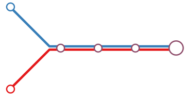
Trunks can be loosely grouped into two categories, “simple trunks” and “complicated trunks.”
Simple trunks are segments of the bus network where routes merge at a single point and share the same travel path between that point and the terminus. Everyone who boards a bus heading towards the shared terminal or alights from a bus heading away from the shared terminus benefits from even headways.
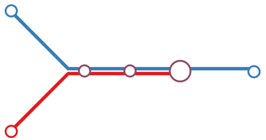
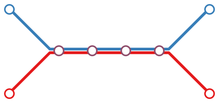
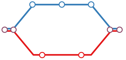
Complicated trunks are segments of the bus network where routes operating on the shared segment diverge at some point, such that some riders may not be able to use the routes interchangeably. This divergence may occur after the end of the main trunk section or in the middle of the route. On complicated trunks, not everyone who boards in the shared segment benefits from even headways.
Figure 1 shows diagrams of simple and complicated trunks and examples of routes that are generally representative of the each type.
Many MBTA bus routes have segments in common with other bus routes, but buses on these routes are often not scheduled with respect to each other or with the primary goal of producing even headways; in either case, uneven headways result. Average passenger wait times may be reduced and distribution of passengers on buses may be improved if headways on these segments were made more even or consistent.
To illustrate the specific issue, consider the hypothetical example shown in Figure 2, where three buses operating on Routes Gray (Trips A and C) and Green (Trip B) arrive at a stop within 10 minutes. In the first scenario, the buses arrive at uneven intervals, and in the second scenario, the buses arrive at even intervals. In both scenarios, we assume that a person arrives at the bus stop each minute, and the first person just misses the first bus. This assumption is merely a simplification for this example.
In this example, when headways are uneven, a passenger who randomly shows up to the stop would wait almost 4 minutes on average. When the headways are even, the average wait for a passenger would be 3 minutes. The passenger load on Trip B in the first, unevenly spaced, scenario would be light and the load on Trip C would be heavy compared to the evenly spaced Trips B and C. The unevenly spaced Trip B would carry only 2 minutes’ worth of arrivals and the unevenly spaced Trip C would carry 8 minutes’ worth of arrivals. In the evenly spaced example, each trip (B and C) would carry 5 minutes’ worth of passenger arrivals.
In the evenly spaced scenario, the first two passengers cumulatively have to wait 6 minutes longer to board a bus than in the unevenly spaced scenario.1 However, their cumulative additional wait time is more than offset by the next three people, who are considerably worse off in the unevenly spaced scenario. In the unevenly spaced scenario, these three riders cumulatively wait an additional 15 minutes over those in the evenly spaced scenario.2 Riders who arrived 5 minutes before Trip C are no better or worse off in terms of wait time in either scenario; however, in the evenly spaced scenario they may experience less crowding on the bus they board.
Figure 1: Diagrams of Simple and Complicated Trunks
Simple Trunks |
Examples of MBTA Bus Routes with |
|
35/36/37 89/101 104/109 214/216 220/221/222 |
Complicated Trunks |
Examples of MBTA Bus Routes with Complicated Trunks |
|
94/96 |
|
106/108 |
|
62/76 87/88 |
Figure 2: Comparison of Uneven and Even Headways on a Trunk
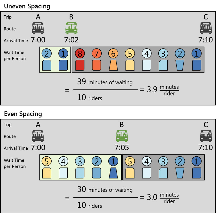
Note: The values displayed inside the circles representing each passenger (that is, the person’s head in the graphic) indicates how long that passenger waits before they board a bus. One passenger arrives each minute.
These formulas do not exactly match the formulas we use later in Section 2.3; they illustrate the problem using a discrete, rather than infinitesimal, number of people. If we used the formulas we describe later (or if we used a finer arrival rate in this example—for example, half of a passenger arrives every 30 seconds), the wait times would be 3.4 minutes in the uneven spacing scenario and 2.5 minutes (half the headway) in the even spacing scenario.
Figures 3 and 4 more concretely demonstrate the problem of unevenly spaced buses on trunk segments by showing the scheduled and the actual distribution of arrivals (shown by the red and blue lines) of buses on several routes operating on a trunk segment. In Figures 3 and 4, the red and blue vertical lines indicate the scheduled departure time for a route at a given timepoint, a stop at which the MBTA records the timeliness of a bus. If the scheduled arrivals overlap, the symbols appear purple.
As shown in Figure 3, on Saturday, inbound trips on Routes 89 and 101 are scheduled to arrive at Winter Hill at nearly the same time. Despite that each individual route is scheduled to operate with regular headways, riders on the trunk section would not experience much benefit in terms of increased service frequency from the existence of multiple routes on the segment; with buses operating so closely on the trunk segment, as long as the service is not crowded passengers boarding on that segment would not perceive significantly better service than if only one of the routes operated. On Sunday, the two routes are scheduled to arrive comparatively more evenly; Route 89 and 101 arrive at this stop with relatively, but not perfectly, even spacing throughout the afternoon.
Figure 4 shows that, on Sundays, Routes 106 and 108 consistently arrive within 10 minutes of each other, followed by a 50-minute gap in service. Separately, each route is scheduled evenly, but together they are not. Shifting the departure time of some trips to reduce the gap in service could improve the customer experience.
Figure 3: Scheduled Arrivals at the Winter Hill Timepoint
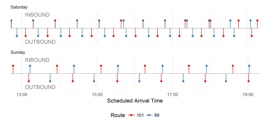
Source: Fall 2016 MBTA Schedule.
Figure 4: Scheduled Arrivals at the Maplewood Street Timepoint
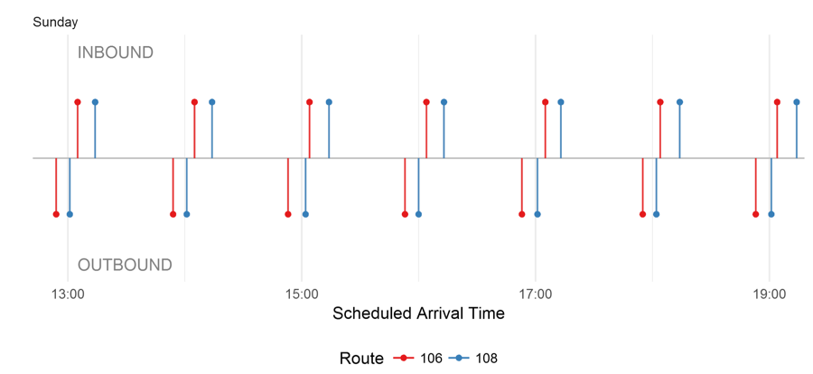
Source: Fall 2016 MBTA Schedule.
The basic methodology we use to estimate the potential benefits of evening out headways on trunks consists of describing trunk sections, determining how long riders on these sections are waiting on average, calculating how much those riders’ wait times could be reduced, and then estimating the number of people who might benefit from the new schedules. (This methodology is summarized in Figure 5.) This analysis relies on two major components: a methodology to determine how long people wait for a bus under a given set of circumstances and stop-level ridership data. For the first component, we adapted a bus schedule performance evaluation methodology used by Transport for London (TfL). This methodology lays out a process for estimating the actual, scheduled, and excess wait times experienced by riders. After calculating the benefit to each rider of a more even schedule, we estimate how many riders would benefit.
We used three primary datasets:
We imported this information into R, a programming language and environment for statistical computing and graphics, in which we completed some of the complicated operations (such as filtering, sorting, joining tables, and iterating the calculations through each branch) on the relatively large dataset. (The GTFS trips by route table contains 920,000 records and 16 fields, and the APC ridership table contains about 270,000 records and 9 fields.)
Figure 5: Data Processing Flowchart
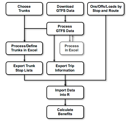
Note: See Appendix A for a more details on the methodology.
To calculate the benefit to passengers from evening out headways, we first need to quantify how long bus passengers are typically waiting for a bus at a stop. TfL uses an excess wait-time (EWT) metric to evaluate the performance of their frequent bus services.3 Essentially, EWT is the amount of wait time passengers experience compared to the wait time they should expect given the schedule. The core function calculates wait times under a given set of scheduled arrival times. EWT is calculated using the following formulas:
Average Actual Wait Time (AWT)=( ∑_(i=1)^N/i=1(Actual Headway)^2 )/( 2×∑_(i=1)^N/i=1(Actual Headway) )
Scheduled Wait Time (SWT) = ( ∑_(i=1)^N/i=1(Scheduled Headway)^2 )/( 2×∑_(i=1)^N/i=1(Scheduled Headway) )
Excess Wait Time (EWT) = AWT – SWT
See below for an example.
Scheduled |
Scheduled (minutes) |
Scheduled |
Actual |
Actual |
Actual |
8:00 |
— |
— |
8:00 |
— |
— |
8:15 |
15 |
225 |
8:05 |
5 |
25 |
8:30 |
15 |
225 |
8:35 |
30 |
900 |
8:45 |
15 |
225 |
8:45 |
10 |
100 |
9:00 |
— |
— |
9:00 |
— |
— |
∑ |
45 |
675 |
∑ |
45 |
1,025 |
|
(× 2) = 90 |
|
|
(× 2) = 90 |
|
AWT=1,025/( 2×45)=11.39 minutes
SWT = 675/(2×45)=7.50 minutes
EWT = 11.39 - 7.50=3.89 minutes
Lower EWT values are more desirable than larger EWT values.
If the number of riders arriving during this time period is known, one could multiply the EWT by the number of riders who use that stop to determine the total EWT. The EWT metric was designed for estimating wait times on relatively frequent services, and it assumes that passengers arrive at the bus stop at a uniform rate during the time period.
To calculate where irregularly scheduled arrivals cause excessive wait times, we modified TfL’s methodology. Instead of calculating the difference between the AWT of actual bus arrivals, we treated the scheduled arrival time as the AWT and we treated a perfectly even schedule as the SWT, which we refer to as the Ideal Wait Time (IWT).4 We calculated IWT and compared it to the SWT to determine how much better the schedule could be. Here, the IWT is equal to half the perfectly even headway, which is equal to the time span of the period under consideration divided by the number of headways we would like to smooth out—or put simply, half the average headway.
Scheduled Wait Time (SWT)=( ∑_(i=1)^N/i=1(Scheduled Headway)^2 )/( 2×∑_(i=1)^N/i=1(Scheduled Headway) )
Ideal Wait Time (IWT) = (Span of Arrivals)/(2 ×Number of Headways)
Excess Wait Time (EWT) = SWT - IWT
See below for an example.
Route |
Scheduled |
Scheduled (minutes) |
Scheduled |
Ideal Arrival Time |
A |
8:00 |
— |
— |
8:00 |
B |
8:05 |
5 |
25 |
8:18 |
A |
8:50 |
45 |
2,025 |
8:36 |
B |
8:55 |
5 |
25 |
8:55 |
A |
9:00 |
— |
— |
9:00 |
|
∑ |
55 |
2,075 |
|
|
|
(× 2) = 110 |
|
|
SWT=2,075/(2×55)=18.86 minutes
IWT = 55/(2×3)=9.17 minutes
EWT = 18.86 - 9.17=9.69 minutes
In this example, if Route A and Route B were scheduled to arrive evenly, the average passenger would save 9.69 minutes (nearly halving the original time) between 8:00 PM and 9:00 PM. If it costs little-to-nothing to shift the 8:05 PM and 8:50 PM trips, while still providing useful service to riders outside the trunk section, this would be a cost-effective way to improve passenger wait times. If the MBTA needed to spend additional resources to reschedule the services, the change may still be worthwhile, but it will be less cost-effective.
Using this methodology, if two buses on two different routes were scheduled to arrive at a stop at the same time, the calculation of wait times based on headways gives no credit for one of the buses. See below for an example.
Route |
Scheduled |
Scheduled (minutes) |
Scheduled |
Ideal Arrival Time |
A |
8:00 |
— |
— |
8:00 |
B |
8:00 |
0 |
0 |
8:10 |
A |
8:30 |
30 |
900 |
8:20 |
B |
8:30 |
0 |
0 |
8:30 |
A |
9:00 |
— |
— |
9:00 |
|
∑ |
30 |
900 |
|
|
|
(× 2) = 60 |
|
|
SWT=900/(2×30)=15.00 minutes
IWT = 30/(2×3)=5.00 minutes
EWT = 15.00 - 5.00=10.00 minutes
In this case, the formula suggests that the IWT is equal to 5 minutes (a headway of 10 minutes). The ideal schedule would have buses arriving at 8:00 PM, 8:10 PM, 8:20 PM, and 8:30 PM. Despite what the tables show, the formula does not specifically indicate the order in which buses on each route should arrive. Route A buses arriving at 8:00 PM and 8:10 PM and Route B buses arriving at 8:20 PM and 8:30 PM would yield the same results as if the Route A and B buses arrived on alternating schedules, one after another.
In order to create a consistent method for estimating the effects of irregular headways regardless of service frequency, we relaxed the assumption that EWT should be calculated only for frequent bus services. In effect, we are ignoring the reality that passenger arrival rates for infrequent services are not uniform; people using these services generally rely on schedules and arrive a few minutes before the bus is scheduled to arrive. However, the actual distribution of arrivals is not particularly important in the context of this study because our focus is on increasing service frequency by reducing service irregularity.
We do not recommend evaluating infrequent bus service in general using the EWT measure because it could result in pressure for buses to arrive early. If buses need to maintain hourly headways, and the previous bus left early, the next bus would need to leave early to maintain an acceptable headway. Early buses leave riders behind.
We calculated EWT in two-hour time blocks. In the following example, our time period was between 7:00 AM to 9:00 AM. During this time period, we counted 6 headways between 6:50 AM and 8:50 AM. Despite that the 6:50 AM trip was outside the time period of concern, we still counted the time between that trip and the first trip in the time period between 7:00 AM and 9:00 AM.
6:50 | 7:10 7:15 7:50 8:10 8:30 8:50 | 9:10 AM
When determining the span over which we should spread those 6 headways, we calculated the time between 6:50 AM and 8:50 AM and divided it by 6, resulting in 20 minute headways. Dividing this headway by two yielded the ideal wait time, 10 minutes. We accounted for the headway between 8:50 AM and 9:10 AM in the 9:00 AM to 11:00 AM time period.
If the time period of concern contained the first trip of a route, we made sure to accurately count the number of headways. In the example below, there were two headways during the 5:00 AM to 7:00 AM time period. The ideal spacing was based on two headways between 5:30 AM and 6:45 AM.
5:30 (First Trip) 6:15 6:45 | 7:15 AM
For trips which span more than one time period, we did not calculate time offsets of our ridership. While we included the service at each stop in the actual time period that it arrived at that stop, we included all passengers boarding on that trip in the time period of the schedule departure time period for the trip whether they boarded during that period or the next time period; if a trip moved into a new time period, its ridership was still counted along with that of the previous period.
See below for an example.
Trip 987123
Stop Schedule Schedule Period Ridership Period
A 6:50 5-7 AM 5-7 AM
B 6:55 5-7 AM 5-7 AM
C 7:00 7-9 AM 5-7 AM
D 7:15 7-9 AM 5-7 AM
This issue only occurs at the beginning and end of each time period. Generally, most of the ridership data should be contained in the correct period, though some ridership will end up in the previous period, and some of the next period’s ridership will end in the current period.5
This problem occurs because the composite APC file and the GTFS file do not perfectly match. Some trip departure times were not found in both files. Aggregating the ridership up to the period level avoided this problem. By using this method, the period-based, APC-derived ridership is still counted at the correct stop, but a portion of it may not be multiplied by the proper travel-time benefit. We chose to use this less precise method because the value added to make the two datasets agree was not worth the cost.
When calculating total travel-time benefits associated with evening out the arrivals of buses, we included all people who boarded and alighted within the trunk.
For simple trunks, where multiple routes join together and end at a common terminal, this calculation works out well. However, for some of the more complicated trunks, where one or more route continues past the shared trunk or where the routes diverge and rejoin, this calculation may include some people who need a specific route and therefore do not benefit from the increased frequency provided by the other route(s). The benefits to passengers on these routes may be overstated. We are more confident in the calculation of benefits associated with simple trunks.
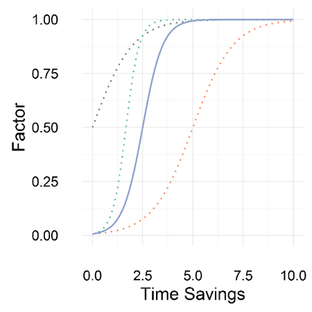
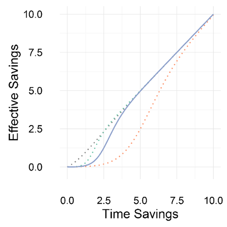
Using the methodology, we observed that in trunks with a large number of bus trips and high ridership, large numbers of riders benefiting from very small wait-time savings translated into very large total wait-time savings. The questionable value of the effort to actually reschedule the trips, given that these areas tend to have relatively short wait times already, plus the idea that anyone would benefit tangibly from a trivial reduction in the amount of wait time, led us to decide to de-emphasize very short time savings. To methodically de-emphasize small wait-time savings, we used a logistic decay function and its associated effective time-savings plot, shown in Figure 6, to transform the time savings.
The logistic decay function takes the following form (the effect of each term is shown in parentheses):
Factor=A/(1+e^(-(B_1+B_2*Time Savings) ) )
A=1 (height of the curve)
B_1= -5 (inflection point of the curve)
B_2=2 (steepness of the curve)
Effective Time Savings = Factor×Time Savings
In Figure 6, we also plotted a few different versions of the logistic decay function to show that there are different curve shapes one could choose. The black curve barely de-emphasizes time savings, the green curve de-emphasizes even smaller wait-time savings, and the orange line de-emphasizes longer wait-time savings. One could also choose entirely different functions to transform wait-time savings (for example, a step function that gives fixed factors to wait-time savings above or below some threshold or a piecewise function that changes at some value).6 Our chosen transformation formula significantly de-emphasizes travel-time savings of under 2.5 minutes.
We show transformed results in the body of this memorandum and untransformed results in Appendix B.
Figure 6: Wait-Time Savings Factors and Effective Wait-Time Savings
We reviewed almost 50 trunk sections of MBTA service. Figure 7 shows the final set of stops we analyzed; some stops are located in multiple trunks. Stops along trunks are spread across the MBTA’s service area.
After following the methodology we outlined, we developed two main tests to determine where evening out headways might provide the greatest benefits:
Figure 7: MBTA Trunk Stops
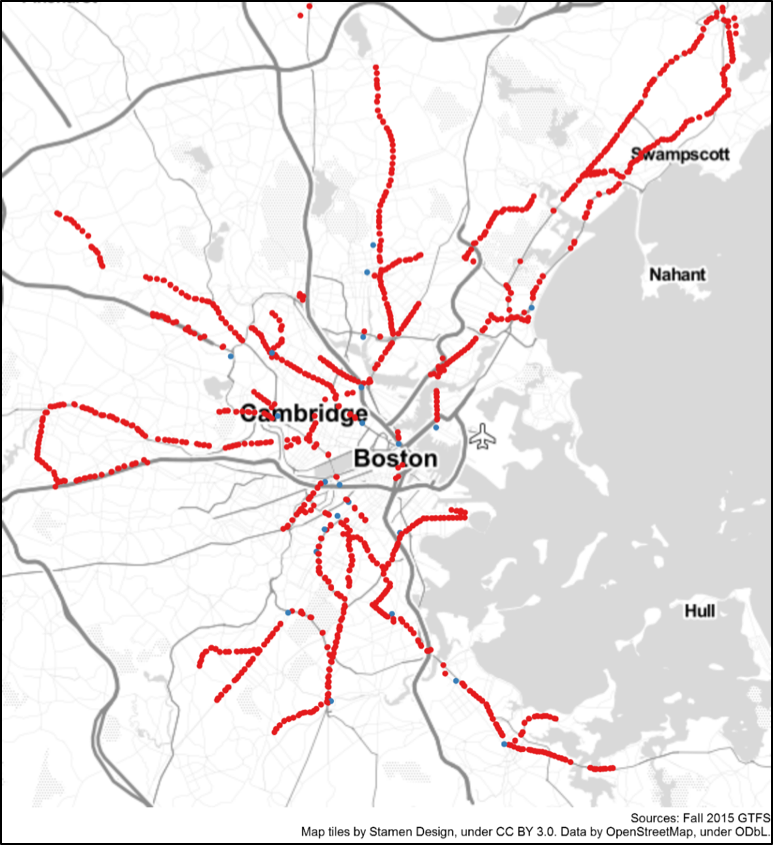
● Stop at a Station
● Other Stops
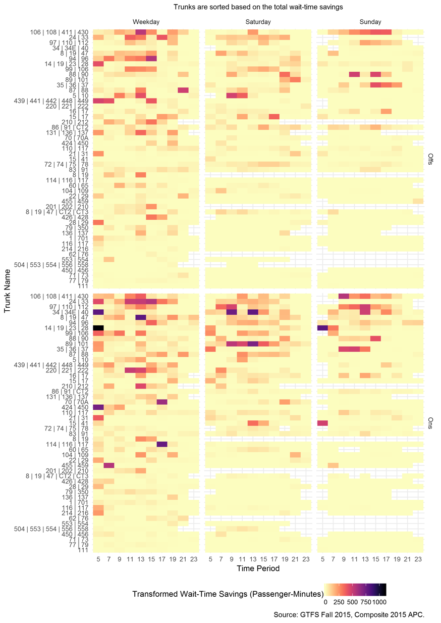
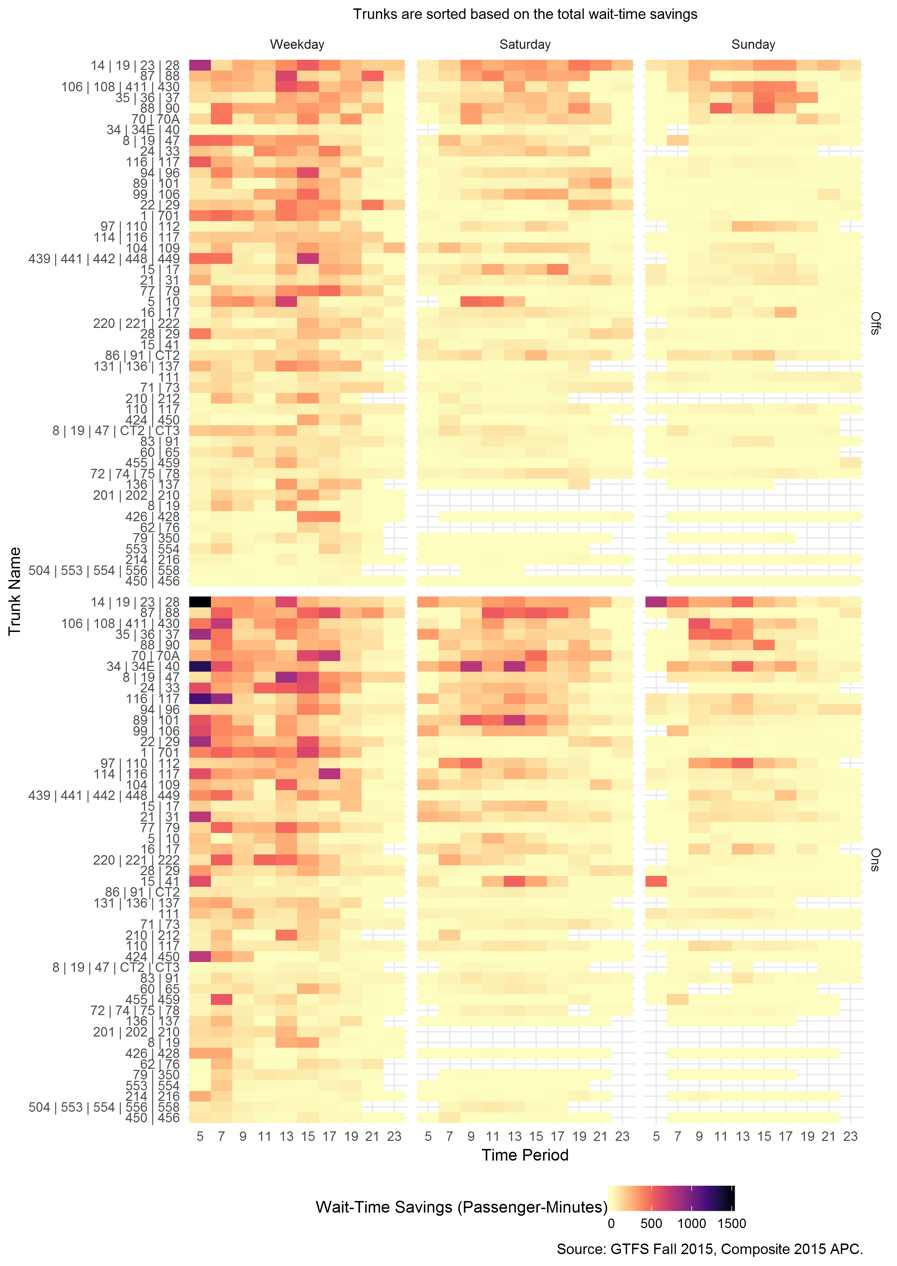
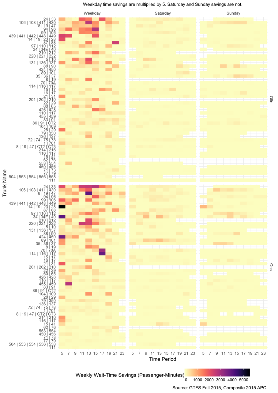
Figure 8 shows that the MBTA could significantly decrease absolute wait times for passengers on several trunks during many time periods. Figure 9 shows the final transformed total wait-time savings by type of day. Most trunk sections have at least one period where riders could benefit from more even headways. Areas in the figures where the color is darker than pale yellow are indications of time periods for which schedules on trunk sections might be better coordinated; a service planner might want to delve deeper to determine the issues preventing better coordinated schedules. Appendix B shows untransformed results, and Appendix C contains results scaled up to a weekly basis, emphasizing the benefits on weekdays.
Figure 8: Excess Wait-Time Savings by Time of Day and Trunk
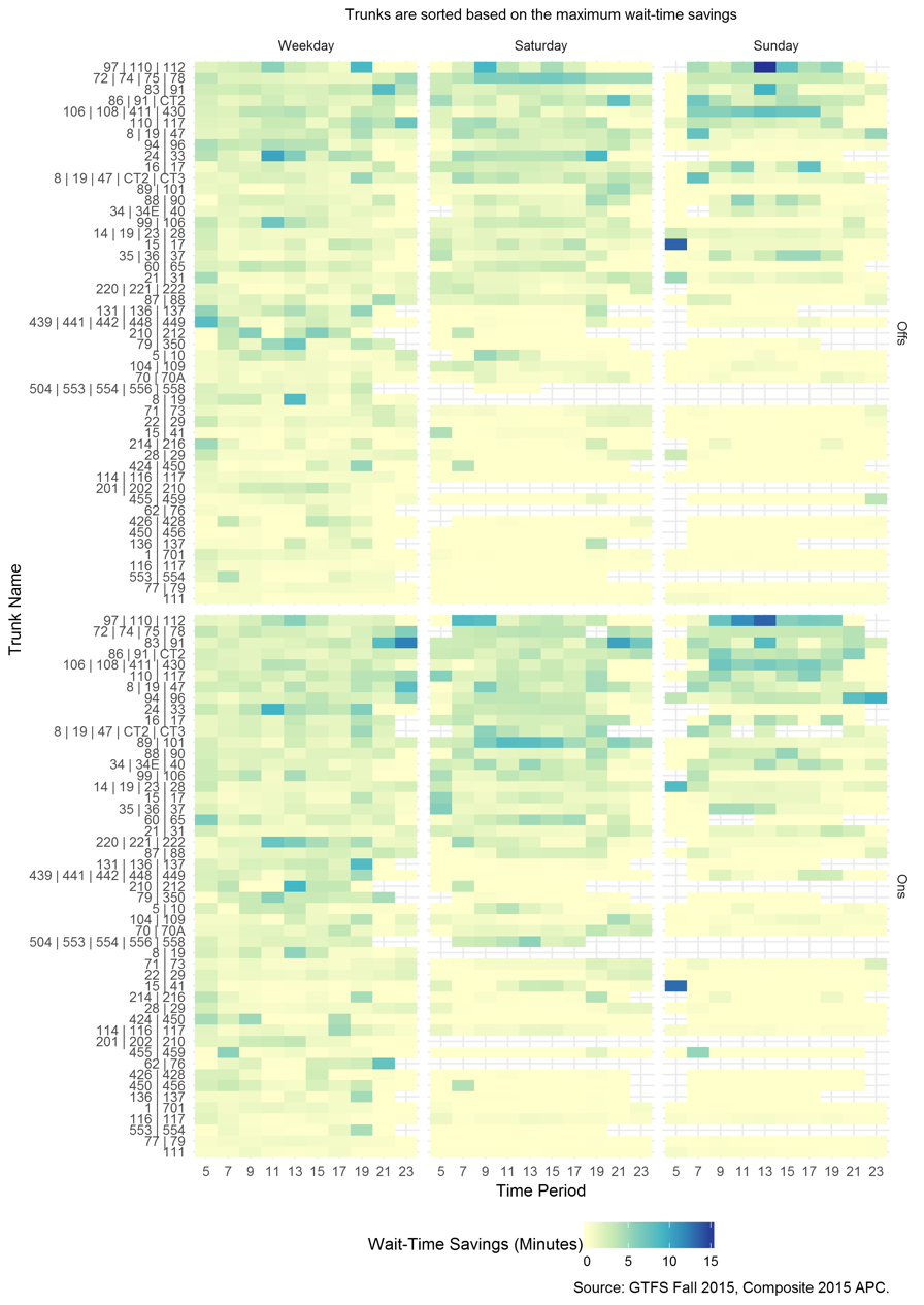
Figure 9: Total Transformed Wait-Time Savings
In terms of absolute, untransformed time savings per passenger, the top 10 period-route combinations (an individual cell in the preceding figures) are as follows:
Trunk |
Start Hour |
Direction |
Day of the Week (DOW) |
Minutes of Savings per Passenger |
97 | 110 | 112 |
13 |
Outbound |
Sunday |
15.41 |
15 | 17 |
5 |
Inbound |
Sunday |
13.52 |
97 | 110 | 112 |
13 |
Inbound |
Sunday |
13.51 |
15 | 41 |
5 |
Inbound |
Sunday |
13.10 |
83 | 91 |
23 |
Inbound |
Weekday |
12.24 |
97 | 110 | 112 |
11 |
Inbound |
Sunday |
11.46 |
83 | 91 |
21 |
Inbound |
Saturday |
10.34 |
24 | 33 |
11 |
Outbound |
Weekday |
10.21 |
94 | 96 |
23 |
Inbound |
Sunday |
9.41 |
24 | 33 |
11 |
Inbound |
Weekday |
9.37 |
In terms of total transformed wait-time savings (savings per passenger multiplied by the number of passengers), the top 10 period-route combinations are as follows:
Trunk |
Start Hour |
Direction |
DOW |
Passenger-Minutes |
14 | 19 | 23 | 28 |
5 |
Inbound |
Weekday |
1,100.2 |
14 | 19 | 23 | 28 |
5 |
Inbound |
Sunday |
796.7 |
8 | 19 | 47 |
13 |
Outbound |
Weekday |
791.0 |
34 | 34E | 40 |
5 |
Inbound |
Weekday |
790.4 |
34 | 34E | 40 |
13 |
Inbound |
Saturday |
781.2 |
114 | 116 | 117 |
17 |
Inbound |
Weekday |
765.4 |
34 | 34E | 40 |
9 |
Inbound |
Saturday |
745.3 |
424 | 450 |
5 |
Inbound |
Weekday |
728.0 |
89 | 101 |
13 |
Inbound |
Saturday |
708.2 |
70 | 70A |
17 |
Inbound |
Weekday |
618.1 |
In terms of total weekly (weekday passenger-minutes are multiplied by five and Saturday and Sunday are multiplied by one) transformed wait-time savings, the top 10 period-route combinations are as follows:
Trunk |
Start Hour |
Direction |
DOW |
Passenger-Minutes |
14 | 19 | 23 | 28 |
5 |
Inbound |
Weekday |
5,501.2 |
8 | 19 | 47 |
13 |
Outbound |
Weekday |
3,955.0 |
34 | 34E | 40 |
5 |
Inbound |
Weekday |
3,952.2 |
114 | 116 | 117 |
17 |
Inbound |
Weekday |
3,827.2 |
424 | 450 |
5 |
Inbound |
Weekday |
3,640.2 |
70 | 70A |
17 |
Inbound |
Weekday |
3,090.7 |
94 | 96 |
15 |
Outbound |
Weekday |
2,787.9 |
24 | 33 |
15 |
Inbound |
Weekday |
2,782.0 |
455 | 459 |
7 |
Outbound |
Weekday |
2,773.3 |
106 | 108 | 411 | 430 |
13 |
Inbound |
Weekday |
2,706.0 |
Note how Saturdays and Sundays no longer appear very high on the list.
In aggregate, if the MBTA were to make all of the headway changes identified, people boarding along trunks during more periods and in more places would have access to frequent service (Figure 10). Approximately 10% more riders benefiting from trunk service would gain access to “frequent” service on weekdays and Saturdays, and approximately 3% more riders would have access to frequent service on Sundays.
Figure 10: Scheduled and Ideal Expected Wait Times by Day of the Week
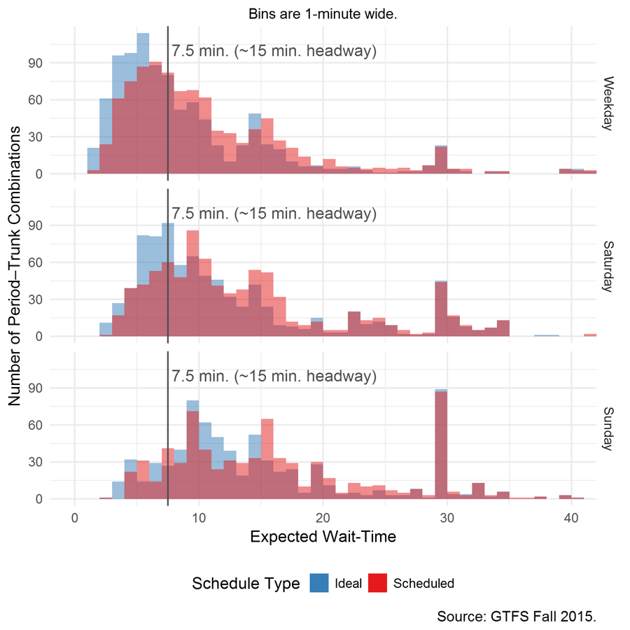
Note: Because some of the trunk sections overlap each other, service planners cannot smooth the headways along every trunk-period combination shown in the figure. Even so, the general benefit, shortening expected wait times, remains valid.
This study focused on where the MBTA might decrease passenger wait times by evening out headways on trunk sections of the bus system. A list of limitations and potential future improvements to our methodology are listed below.
The steps of our methodology are listed below.
1 In the evenly spaced scenario, the first two passengers wait 5 minutes and 4 minutes, respectively, while in the unevenly spaced scenario they wait 2 minutes and 1 minute, respectively.
2 In the evenly spaced scenario, the third, fourth, and fifth passengers wait 3 minutes, 2 minutes, and 1 minute, respectively, while in the unevenly spaced scenario they wait 8 minutes, 7 minutes, and 6 minutes, respectively.
3 TfL uses the EWT calculation when 5 or more buses are scheduled to arrive per hour. This is equal to a headway of 12 minutes or better. See this TfL site for more information about their metric: https://www.gov.uk/government/uploads/system/uploads/attachment_data/file/489755/measurement-template.pdf
4 IWT is considered ideal in terms of minimizing passenger wait time.
5 We initially tried to join each trip based on its departure time, a process that would take care of the arrival-time offsets, but because a large number of the departures did not join properly, it did not seem worthwhile to spend resources fixing the problem. We chose to use a slightly less precise, but more forgiving, method where we joined the total “ons” and “offs” occurring during a period to each stop—eliminating the need to join specific trip departure times.
6 We chose this functional form because it allows us to easily change the shape of the curve to fit our needs. With a single function, we can significantly de-emphasize small time savings while not affecting large time savings.